


 MENU
MENUI’m Melinda Horne, a master’s student in the Hydrology program in the Earth and Environmental Sciences department of New Mexico Institute of Mining and Technology. My research involves analyzing a geothermal reservoir in south-central New Mexico.
The system was modeled in Fortran by Dr. Mark Person, who is my advisor. It is a two-dimensional model capable of simulating groundwater, heat and solute transport, as well as tectonic evolution and petroleum generation. With no surface expression, it is a blind geothermal reservoir, however there is one geothermal well with temperatures of 99 C at 371 m depth and a total dissolved solid of 1900 mg/L.
This geothermal reservoir is unique because it displays hotter temperatures at shallower depths – called a temperature inversion. Another unique feature is that it is located at the nexus of three hydrologic drainage divides and a buried geologic uplift. We believe that it is a steady-state system with a complex three-dimensional flow.
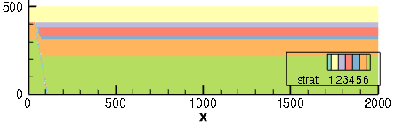
Figure 1. Model domain with geologic unit assignments. Purple is a hot aquifer and blue is a cool aquifer. The light blue line offsetting the units is the fault that is the geothermal fluid conduit.
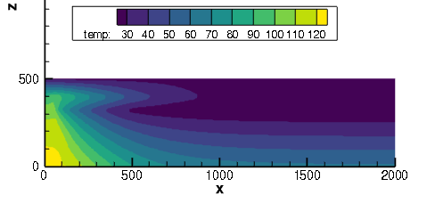
Figure 2. Best-fit heat transport run with uncoupled temperature effects on density. This is after 10,000 years of flow. Input temperature is 120 C and flux is 200 m/yr. The cooler aquifer has a temperature of 30 C and 0.01 m/year flux.
Determining Temperature and Flow Rate
Our first challenge was to determine the flow rate and temperature of the geothermal reservoir and regional flow system. To do this, we used Tecplot 360 to display the 2D model with temperature, heat and solute concentration contours. Then we extracted a temperature-depth profile from the model output at the location of the geothermal well to match the well’s temperature-depth data (see Figure 3).
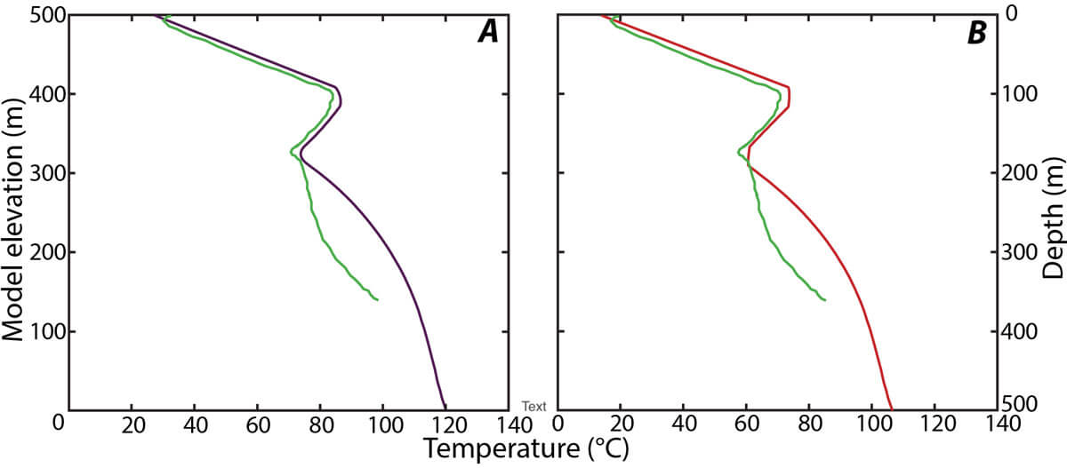
Figure 3: Compares data (green) to best-fit coupled (red) and uncoupled (purple) simulations. This
demonstrates that coupled and uncoupled simulations have different best-fit results that most likely
result from increased mixing from the effects of coupled temperature and density effects.
Determining Salinity
The second challenge was to image the geothermal upflow zone and determine the salinity and lateral extent of the system. We extracted salinity in Tecplot 360 and then post processed in R to convert from model salinity to formation resistivity. The 2D formation resistivity plots were used to compare to the formation resistivity data we collected with surface electrical surveys (transient electromagnetics). The collected data, which are also 2D plots, were interpolated and contoured in Tecplot 360.
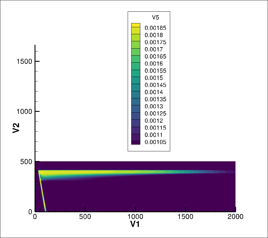
Figure 4. Salinity contours across the model domain. The fault base has a salinity of 3,000 mg/L and the initial condition of the model has a salinity of 1,000 mg/L.
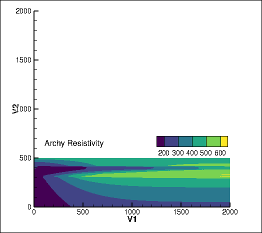
Figure 5. Archie’s Law resistivity across the model domain. This is obtained from extracting the salinity, post processing in R, and then uploading the subsequent Archie resistivity to Tecplot 360 to display.
Why I Use Tecplot 360
I have been using Tecplot 360 on and off for about two years, and there are many features that I find useful. These were especially helpful for my research:
- Extracting Data – Without the ability to extract a precise line, I would not be able to match the geothermal temperature-depth profile.
- Customizing contour ranges and colors – very helpful for communicating my work!
- Reading in data – including whole-mesh datasets.
- Exporting the model – using the write data feature, post processing it, and then reading the data back into Tecplot 360 to display it.
Tecplot 360 is extremely easy and intuitive to use and has been an irreplaceable tool for my master’s research.