Visualizing Higher-Order Elements – Part 1: A Primer
This blog was written by Dr. Scott Imlay, Chief Technical Officer, Tecplot, Inc.
“DON’T PANIC!” Douglas Adams, Hitchhikers Guide to the Galaxy
In the next few blogs I’ll discuss our recent research on the visualization of results from higher-order element computational fluid dynamics (HOE CFD). If you are not one of the practitioners of this specialized form of CFD you may be asking “what?” If so, it’s OK, please just heed the advice of Douglas Adams and “DON’T PANIC!”
First, a quick primer on partial differential equations. Again, “DON’T PANIC!”
The behavior of a fluid flow is described by a set of partial differential equations which relate how the local state of the flow (density, momentum, energy; or alternatively pressure, temperature, velocity) changes over time and space. The simplest of these equations is the conservation of mass (continuity) equation

where ρ and u are the density and velocity of the fluid at a point in space and time (x and t). This equation is the mathematical version of the statement “mass cannot be created or destroyed”, or “if more mass flows into a region than flows out, the density must increase over time.”
If you’re not familiar with symbols in this equation, DON’T PANIC!
The ∂ symbol represents a partial derivative and ![]() is the rate at which the density, ρ, is changing in time. Likewise,
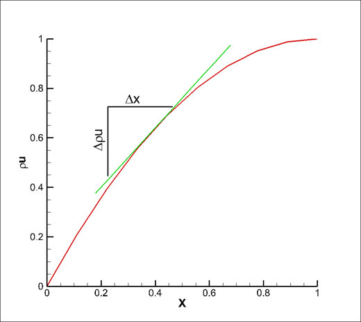
is the rate at which the density, ρ, is changing in time. Likewise, ![]() is the rate at which momentum (density times velocity) increases with increasing spatial dimension x. Another way to think of the partial derivative is as the slope of the curve:
is the rate at which momentum (density times velocity) increases with increasing spatial dimension x. Another way to think of the partial derivative is as the slope of the curve:

Figure 1. ∂ρu/∂x is the rate at which momentum (density times velocity) increases with increasing spatial dimension x, which is the slope of the curve.
In the above chart the red line is the variation of ρu with x and the slope (change in ρu over change in x) of the tangent green line is ![]() at the point of tangency.
at the point of tangency.
Approximating the Derivative
Of course, we don’t generally know a functional form for ρu in terms of x, so we need to approximate the derivative. This is where the order of accuracy comes into play. In solving these partial differential equations we use a grid, with Δx being the grid spacings between grid points. If our approximation to the derivative, call it ![]() , has an error term proportional to Δxn we call it an n-th order accurate scheme. For example, a second order scheme would approximate the derivative with an error proportional to Δx2
, has an error term proportional to Δxn we call it an n-th order accurate scheme. For example, a second order scheme would approximate the derivative with an error proportional to Δx2

where the … represents terms containing higher exponents of ∆x like Δx3, Δx4, and so on. As the grid spacing Δx gets smaller the error terms with exponents higher than second order will vanish more quickly than the leading Δx2 term, so the approximation is called second order accurate. The majority of CFD codes are second-order accurate.
Higher-order Schemes
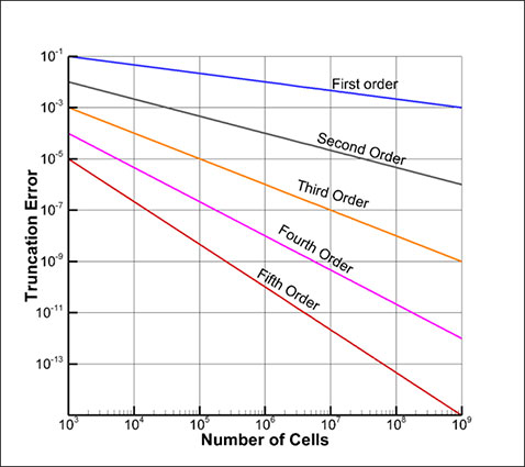
Higher-order schemes have a leading error of greater than second order. For example, a third-order scheme will have a leading error term of Δx3. As the order of the scheme gets higher, the approximation error drops more rapidly as the grid spacing Δx gets smaller. A higher-order scheme gives a more accurate solution than a second-order scheme with a given grid spacing. Alternatively, you can say that the grid spacing doesn’t need to be as small to get a desired level of accuracy. It is the ability to use a coarser grid to get the same level of accuracy that makes the higher-order schemes attractive.

Figure 2. It is the ability to use a coarser grid to get the same level of accuracy that makes the higher-order element schemes attractive.
Finite-element Methods
For finite-element methods, the variation of the solution over the element is generally approximated as a polynomial with unknown coefficients. For example, in two-dimensions, the element shape may be triangular with a linear variation of solution over the triangle. The goal of the finite-element method, therefore, is to solve for coefficients of the polynomials for all elements in such a way to give the best approximation to the solution of the partial-differential equations.
Enough about the method, let’s focus on the finite-elements themselves!
Why Use Higher-order Elements?
The degree of the polynomial determines the order of accuracy of the scheme (at least the spatial derivatives). For example, linear elements are second order accurate, quadratic elements are third-order accurate, and cubic elements are fourth-order accurate. In general, if p is the degree of the polynomial approximation then p+1 is the order of accuracy.
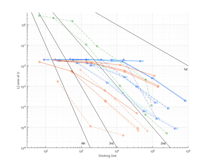
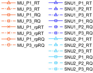
Why use higher-order elements? In short, for a large class of problems, HOEs achieve a desired level of accuracy with less computation expense. The following chart (Figure 3) from the AIAA Higher-Order Workshop shows how this is true. The horizontal axis of this chart is “work units” (how much computational resources the code uses) and the vertical axis is the solution accuracy (not order-of-accuracy, but how close the solution is to the correct solution). As you can see, the “_P3_” results for each of the codes tend to perform better than the “_P1_” or “_P2_” results. Here “P3” indicates a cubic polynomial which would yield a fourth-order accurate scheme. Note that in the chart below, down is more accurate.

Figure 3. Higher-order elements achieve a desired level of accuracy with less computation expense. This chart, from the AIAA Higher-Order workshop, shows how this is true. The horizontal axis of this chart is “work units” (how much computational resources the code uses) and the vertical axis is the solution accuracy (not order-of-accuracy, but how close the solution is to the correct solution). Down is more accurate.

Legend for Figure 3.
Unsteady Flows
Unsteady flows with propagating vortices are the class of flows that benefit the most from higher-order methods. This is the type of flow you often get with large-eddy simulations, which are becoming more popular as computers get more powerful. For this reason, the usage of higher-order methods will likely increase in the future. Visual Analysis codes like Tecplot 360 need to be ready.
In the next blog I’ll discuss the complex nature of higher-order finite-element data. See all blogs on higher order elements.
Subscribe to Tecplot 360
Get notified when the next blog is posted!


