This blog was written by Dr. Scott Imlay, Chief Technical Officer, Tecplot, Inc.
In this series of blogs, I discuss the results of our research on visualizing higher-order finite-elements. The first blog on this topic was A Primer on Visualizing Higher-Order Elements. The second was on the Complex Nature of Higher-Order Finite-Element Data. And the third was on Visualizing Isosurface Algorithms for Higher-Order Finite-Elements.
In this 4th blog of the series, I take a look at a technique for visualizing higher-order surface elements.
Carry on, my wayward son
There’ll be peace when you are done
Lay your weary head to rest
Don’t you cry no more– Chorus of “Carry On Wayward Son” by Kansas
Fluid Dynamics of Driving Cross Country
I’m driving through the South Yakima Valley in our “new to us” motorhome and this is playing on the stereo. On this day, these words speak to me in multiple ways. First, tomorrow would have been my daughter’s 35th birthday. This was the theme song to one of her favorite TV shows and could have been the theme song for her final weeks of life. “Carry on my sweet daughter, there’ll be peace when you are done!” Second, we are currently driving to the Grand Canyon where I’ll join some friends to run from the South rim to the North rim and back (about 50 miles). I’ll definitely need some prodding to “carry on”, I’ll be very “weary” at the end, and there may be tears. But, most immediately, I’m currently driving with a 40 mph crosswind.

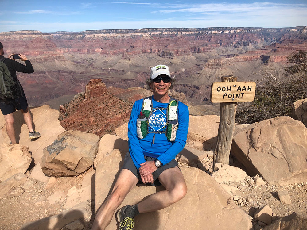
As I write, we are driving to the Grand Canyon where I’ll join some friends to run from the South rim to the North rim and back (about 50 miles).
When a gust hits the motorhome leans uncomfortably to the left and I need to steer right to keep it in the lane. Then we pass into a calmer area behind a hill and the motorhome veers to the right. I contemplate stopping until the wind dies but I know they will subside in about 30 miles, so I “carry on.” I’m using my fluid dynamics knowledge to estimate when the crosswind will subside slightly (high bank on the windward side) and when it will increase (gullies through the bank). I come up on a bridge over a gully and prepare for an increase in wind, but it actually reduces a little. What? A PhD and nearly 40 years of experience in fluid dynamics and it can still surprise me.
Turbulent Boundary Layers
I’m driving in a turbulent atmospheric boundary layer, and the nature of the turbulence is highly dependent on the geometry of the terrain. In the atmosphere, this boundary layer is hundreds or thousands of feet thick, but on an airplane it may be a fraction of an inch thick. When doing a CFD computation of the air flow around an airplane, especially doing a large-eddy simulation of a direct numerical simulation of the turbulence, the geometry must be precisely described. For standard second-order accurate CFD calculations, this is done by using an enormous number of surface elements, but for higher-order element methods, the surface elements (or the side of the volume element defining the surface) generally must be curved.
For higher-order finite-element surfaces, the geometry (x,y,z coordinates of any point on the surface) is defined for each element by polynomials in terms of the local surface coordinates (r,s). If the same polynomial type and order is used for the solution and the geometry, it is called isoparametric. If a lower order polynomial is used for the geometry than compared to the solution, it is call subparametric. If higher, it is superparametric. In any case, if the same type of polynomial functions are used for geometry and solution, and then similar visualization techniques can be used as well.
Technique for Visualizing Higher-Order Surface Elements
Our technique for visualizing higher-order surface elements is very similar to our technique for higher-order volume elements. We use hierarchical subdivision of the surface elements. On each level of subdivision, triangles are subdivided into four sub-triangles and quadrilaterals are subdivided into four sub-quadrilaterals. The hierarchical subdivision of the surface elements continues until the resulting set of linear elements is a good representation of the curved polynomial surface.
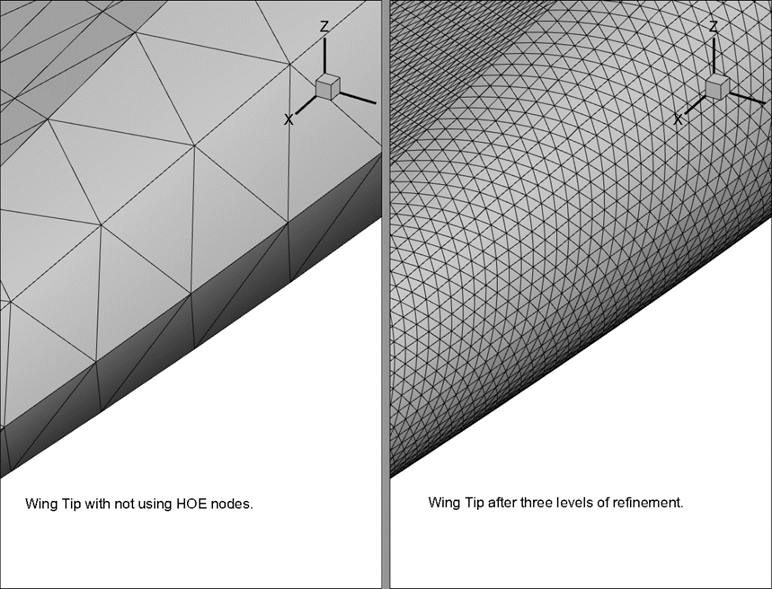
The figure below shows how this works for quadratic triangles defining the surface of an ONERAM6 wing. The image on the left is the surface created if you throw out three additional high-order nodes and just treat the quadratic elements as linear elements. The image on the right is after three levels of subdivision. The refined surface is a much better representation of the actual surface.

Wing tips with and without HOE nodes. See all HOE blogs.
I will have at least one more blog on visualization of higher-order finite-element results, although I’m not yet sure what it will cover. Check back to find out! Or Subscribe to Tecplot.


