How to Create and Unwrap a Cylindrical Slice Using Tecplot 360

With axisymmetric geometries you may want to extract a cylindrical region to understand the properties of certain scalar values as a function of Theta. This article will help you understand how to create a cylindrical slice and how to properly display it in Tecplot 360.

For this article we’ll use a single timestep of a CONVERGE internal combustion simulation, which is included in the Tecplot 360 Getting Started Bundle.

The key components to creating this plot are:

• Compute Radius and Theta variables
• Create and extract an iso-surface at a constant radius
• Plot the extracted iso-surface in a 2D plot with Theta on the X-Axis
• Enable Value Blanking to eliminate cells which span the periodic boundary where Theta goes from -Pi to +Pi (this is explained in detail below)

So, let’s start…

Loading the Data and Computing Radius and Theta

The first step is to load the data and compute the new variables we’ll need to extract the iso-surface and to “unwrap” it in a 2D plot.

1. Go to File > Load Data and select “ICE\ICE000045_-1.60894e+02.plt” from the Getting Started Bundle
2. Go to Data > Alter > Specify Equations and enter the following formulas:
   {Radius} = sqrt(X*X+Y*Y)
   {Theta} = atan2(X,Y)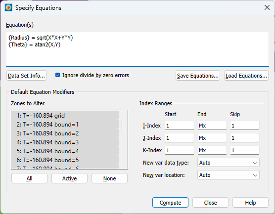
3. Activate Iso-Surfaces and define an iso-surface at Radius = 0.0278. You may need to visit the Contour Details dialog to change the Contour Group variable assignment. You should be able to make a plot similar to the one seen here:
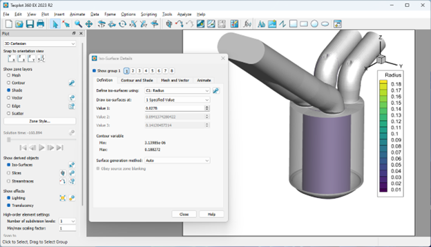
4. Use Data > Extract > Extract Iso-Surfaces to create a new zone from this iso-surface

Unwrapping the Cylindrical Slice

Now that we have a new zone from the iso-surface, which represents a constant radius, we need to unwrap that surface in a 2D plot using the Theta variable. To do this follow the steps here:

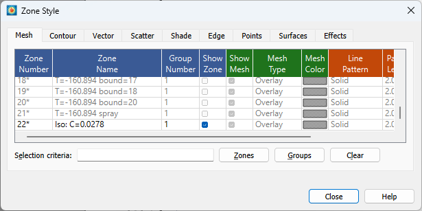
1. In the Zone Style dialog, deactivate all zones except for the extracted iso-surface
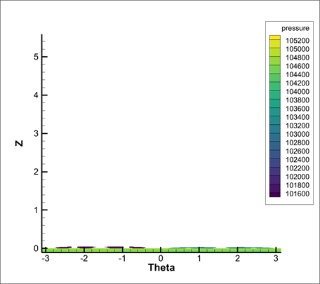
2. Switch the Plot to 2D Cartesian and use Plot > Assign XY to select Theta and Z and the X and Y-axes respectively. You should now have a plot that looks something like this:
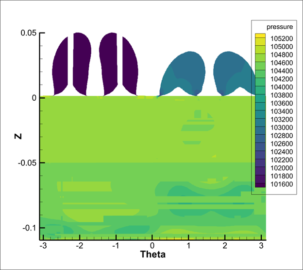
3. Change the Axis Dependency to Independent via the Plot > Axis dialog , and then use View > Fit to Full Size to fit the data. You should now have a plot that looks something like this:
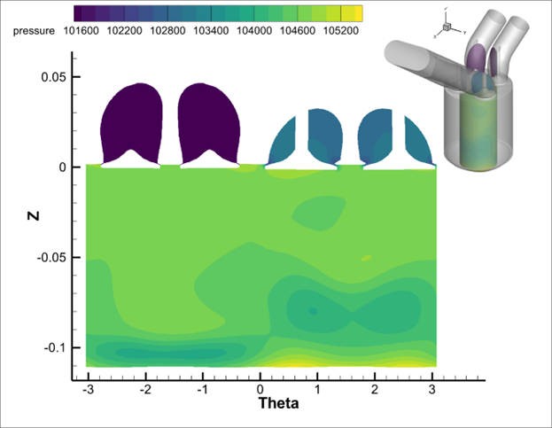
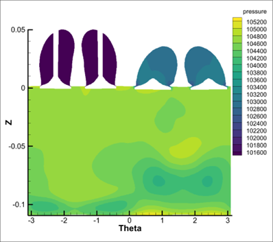
4. We’re almost there! You’ll notice some interference in the plot. We’ll explain this below, but for now – just go to Plot > Blanking > Value Blanking and set it up to blank out cells where Y <= -0.02779 . Notice that the interference is gone. 

Explanation of the Need for Value Blanking

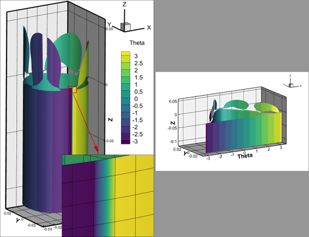
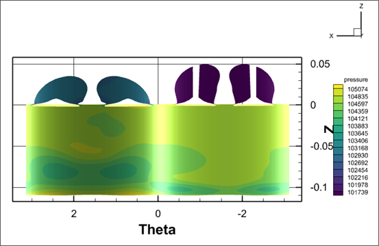
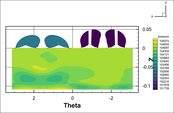
When computing the Theta values, there is one strip of cells where the value of Theta transitions from -Pi to +Pi. This strip of cells effectively contains all values of Theta and will therefore be stretched across the entire 2D domain. In the image below, you can see a visual representation of this. The plot on the left shows the cylindrical slice colored by Theta, and the strip of cells which represents all values of Theta can clearly be seen. In the plot on the right, we’ve assigned the X-axis to the Theta variable, and again it can be seen how that strip of cells is stretched across the entire Theta domain.

In 2D plots, there is only the concept of an X and Y variable, so that strip of cells which is easily seen in 3D space, get drawn on top of one another in 2D space. To eliminate those cells from the drawing we use Value Blanking to remove the cells. In this case those cells correspond with the Y-minimum value, which is why we use Value Blanking of the Y-variable at the Y-minimum value (plus a small epsilon).

An Alternative to Using a 2D Plot…

Another option for plotting would be to use a 3D plot, with Theta on an axis (like we’ve drawn above). Just make sure to rotate the plot correctly, such that the ‘stretched’ cells are in the back. You’ll also want to turn off Lighting on the Plot Sidebar. 

Lighting Effect On

Lighting Effect Off

Using PyTecplot to Automate the Process

Available on the Tecplot GitHub site is a script which automates this process: https://github.com/Tecplot/handyscripts/blob/master/python/AnnularSlice.py

To use this script, follow the instructions here:

1. Go to File > Load Data and select “ICE\ICE000045_-1.60894e+02.plt” from the Getting Started Bundle
2. Enable PyTecplot connections via Scripting > PyTecplot Connections…”
3. In a command prompt, run the AnnularSlice.py script
   Windows: python -O AnnularSlice.py
   Linux/macOS: /path/to/360/bin/tec360-env — python -O AnnularSlice.py
4. Follow the prompts as pictured:

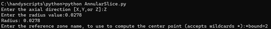
At the time of writing this article, the script will then perform nearly all the manual steps listed in this article. The result sets up Value Blanking to use the minimum Y-value, which is not sufficient for this case, so you’ll have to add a small epsilon to the value blanking constraint yourself (i.e. Y <= -0.02779).

See this tutorial in action by watching our video walkthrough below!