


 MENU
MENUThe computation of derivatives is an important part of CFD post-processing. Derivatives of scalar variables such as temperature and chemical composition drive physical processes such as heat conduction and diffusion. Likewise, derivatives of velocities are responsible for things like shear stress and drag forces of aircraft. With the release of Tecplot 360 2024 R1, we have introduced the Green-Gauss method for computing derivatives as a Beta feature, available via the macro language only as such:
$!AlterData
FEDerivativeMethod = GreenGauss
Equation = '{dudy_gg} = ddy({u})'
Why Green-Gauss Derivatives?
For decades, Tecplot 360 has computed derivatives using the moving least-squares (MLS) method. In this method, the data values of the function at nodes (or cell-centers) near the node of interest are fit to a quadratic polynomial from which the derivatives are computed analytically. For most finite-element grids, the MLS method yields accurate estimates of the derivatives. However, for highly stretched and/or skewed regions of grids, it can yield a poor estimate of the derivatives.
Many CFD codes use the Green-Gauss formula to compute an estimate of the derivatives. The Green-Gauss method computes the derivatives using surface integrals and, therefore, is considered to be less sensitive to highly stretched and/or skewed grids.
As grids get denser, we find that the cells near the boundary become more and more stretched – hence it’s important that Tecplot 360 allow use of method that provides a high degree of accuracy in these regions – typically the most important regions as they’re within the boundary layer. For reference, see CRMHL_Wingbody_5v.cgns here: https://hiliftpw.larc.nasa.gov/Workshop5/grids_downloads_case1.html. This is on the small side of the grids used for the High Lift Prediction Workshop with only 36M cells and you can already see how stretched the cells are near the surface.

Green-Gauss Formula
The Green-Gauss theorem states that the surface integral of a scalar function, ∅, is equal to the volume integral (over the volume bound by the surface) of the gradient of the scalar function.
 The left side of this equation is the average gradient within the volume and the right side can be approximated as a summation of the average scalar value in each face times the face’s surface vector. The resulting equation is

Since the components of the gradient vector are the partial derivatives in the spatial dimensions, this equation can be used directly to compute derivatives. We need only define a suitable volume V around the node of interest.
Defining the Volume
The best volume seems to be one that minimizes the number of surrounding nodes used (a compact stencil). In a two-dimensional finite element grid containing triangles this means using all the nodes of triangles containing the node of interest (the node where you are computing the derivative). If the grid contains quads, it means eliminating the node opposite the node of interest, creating a triangle from the remaining nodes.

If the node of interest is on a boundary, the boundary surfaces (edges in 2d) containing that node are included in the volume definition.

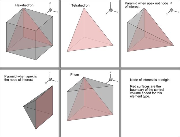
In three dimensions it is a little more complicated. Again, we wish to use a compact stencil so, for bricks and prisms, we use the tetrahedra defined by those nodes directly connected by an edge to the node of interest. For tetrahedra, the contribution to the control volume boundary is just the face opposite the node of interest. The most complicated element is the pyramid, where the full quad opposite the apex must be used to compute the derivative at the apex node. Note that, since the pyramid is the only element where more than a tetrahedron is added, it is often required to add other triangular surfaces of the pyramid to complete the control volume surface.
Results and Comparisons with Moving-Least-Squares
For a highly stretched and curved grid in the figure below, the skin friction coefficients from FE-Brick Green-Gauss derivatives compare favorably with those from IJK-Ordered derivatives, which have been shown to be accurate. In comparison, the skin friction coefficients from MLS derivatives are substantially different in this case, particularly near the leading edge. This is due to MLS using a broad stencil with data from nodes further out along the curved grid than Green-Gauss.


Data courtesy: Mauro Minervino, Research Engineer at the Italian Aerospace Research Centre
Conclusions and Recommendations
For smooth well-behaved grids, moving-least-squares will give a good, and sometimes better, approximation for the derivatives and will likely remain the preferred option. However, if you have highly stretched and/or skewed grids, the Green-Gauss derivatives are likely to be more accurate and, therefore, the better option.
Computation of derivatives with Green-Gauss is currently about 20% slower than Moving-Least-Squares, but optimizations are possible that should make the performance roughly the same. There is no significant difference in memory usage between Green-Gauss and Moving-Least-Squares.
If you wish to try using Green-Gauss derivatives, it is available as a beta feature in Tecplot 360 2024 R1 for nodal data in finite-elements (not high-order or polyhedral). Moving-least-squares is the default method in 360 2024 R1 and 360 will fall back to MLS for data types that don’t support Green-Gauss.
You will need to run a macro like this to compute the Green-Gauss derivatives:
$!AlterData
  FEDerivativeMethod = GreenGauss
  Equation = '{dudy_gg} = ddy({u})'
In future versions of Tecplot 360, there will be an option in the user interface to select Green-Gauss derivatives.
References
“Gradient Computation”, CFD Online, https://www.cfd-online.com/Wiki/Gradient_computation.